<?xml version="1.0" encoding="utf-8"?><feed xmlns="http://www.w3.org/2005/Atom" xml:lang="en"><generator uri="https://jekyllrb.com/" version="3.10.0">Jekyll</generator><link href="https://davidclarance.github.io/feed.xml" rel="self" type="application/atom+xml" /><link href="https://davidclarance.github.io/" rel="alternate" type="text/html" hreflang="en" /><updated>2026-09-07T17:09:03+00:00</updated><id>https://davidclarance.github.io/feed.xml</id><title type="html">David Clarance</title><subtitle>Notes, essays and occasional half-formed thoughts.</subtitle><author><name>David Clarance</name></author><entry><title type="html">Birding in Weymouth</title><link href="https://davidclarance.github.io/writing/birding-in-weymouth/" rel="alternate" type="text/html" title="Birding in Weymouth" /><published>2026-01-09T00:00:00+00:00</published><updated>2026-01-09T00:00:00+00:00</updated><id>https://davidclarance.github.io/writing/birding-in-weymouth</id><content type="html" xml:base="https://davidclarance.github.io/writing/birding-in-weymouth/"><![CDATA[<p>Weymouth is new to me. I googled places to bird in the winter and Weymouth came up as a relatively good location. I checked train tickets and there seemed to be a direct connection from London, so I just decided to go ahead! I’m so glad I came. What an incredible part of the country to go birding in. I didn’t have personal transport for the trip, so I mostly just walked or used the bus. According to my Garmin, I walked about 60 km in around four days (Thursday was a complete washout). So if you enjoy walking, there’s loads to do.</p>

<p>Here’s the the complete ebird list: <a href="https://ebird.org/tripreport/461318">https://ebird.org/tripreport/461318</a></p>

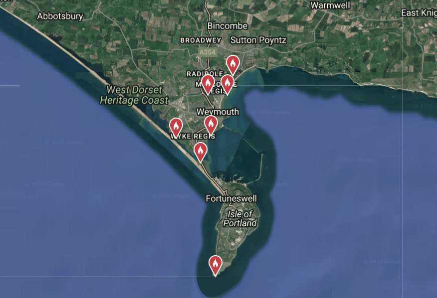
<p><img src="/assets/writing/birding-in-weymouth/trip-map.png" alt="Map of the Weymouth birding trip" /></p>

<h2 id="day-1">Day 1</h2>

<p>I took the train from London Waterloo and reached Weymouth at about 1 PM. I dumped my bags at the Airbnb and headed straight for the Lodmoor wetlands. It was cold, but so rewarding! I had brilliant views of a bullfinch pair and a firecrest as I entered. What a joy! Some of the highlights were seven (!!) snipe, literally 100 green-winged teal, and the beautiful, beautiful northern lapwing. Over the reedbeds, a nice male western marsh harrier hovered and hunted. A Cetti’s warbler came out and did its thing. Overall, a super productive evening. I went home exhausted and crashed.</p>

<p>One curious thing I don’t think I’ve seen anywhere else were how the many European Herring gulls hunted. They would pick up shells (presumably with clams) from the water / beach, fly high and then drop them on the payment. The shells would split and the gulls would feed on them. What’s even more weird is that I didn’t see the crows copying that behavior. Crows are incredibly smart so I was quite surprised by that and wonder why that’s the case. Or maybe I didn’t pay enough attention to it?</p>

<h2 id="day-2">Day 2</h2>

<p>I was up early, made some coffee and a quick cheese sandwich, and planned the day. An interesting geographical feature of Weymouth is the Fleet. The Fleet is the UK’s largest brackish water lagoon. The start of the Fleet is the pebbly storm overflow called Chesil Beach. From lists and trip reports, it seemed to have a strong gathering of birds, so I figured I could get a bus close by and walk.</p>

<p>As I set out, I saw a beautiful peregrine hunting in the morning light. It was FREEZING when I reached the beach, but my first sighting was a lifer: a pair of European shags. As I continued to walk, I was met with dozens of brant. Other highlights that morning included oystercatchers, ruddy turnstone, and skylark. As the sun began to come up, there was a lot more activity. Loads of dunlin and some black-bellied plovers as well.</p>

<p>At around 10:30, I went to the lovely café and had some coffee and a massive slice of apple cake. It was warm and cozy and full of birding people. I then went out for another look to see if anything interesting arrived as the tide started to go out. While standing and scanning, I heard three senior birders discussing the day. When they finished chatting, two of them left, so I asked the remaining gentleman where the grey plovers were. He very kindly pointed them out to me. We struck up a conversation, and it turned out he knew the parents of a person I knew from Kenya (for my Kenya birding homies, he knew Colin Jackson’s parents from back in the day). What an incredibly small world! His name is Nigel and we ended up chatting a bunch. He used to be a vicar and is now living his happy retired life birding Weymouth and the surrounding areas.</p>

<p>Since I didn’t have any transport, Nigel very kindly let me tag along with him to Portland, where we saw common murre, a common gannet, and the usual gulls. As we were preparing to leave, Nigel was convinced there would be purple sandpipers along the coastline. We scanned loads and finally found them. Four beautiful purple sandpipers frolicking in the overflow.</p>

<p>Nigel very kindly dropped me back in Weymouth again. I ate a quick sandwich and made my way back to Lodmoor. I found all the usuals, but also got my first glimpse of a water rail.</p>

<p>Tired and hungry, I got home, chewed Tvisha’s brain about all the birds I’d seen, and crashed.</p>

<h2 id="day-3">Day 3</h2>

<p>The next day I was up again and ready to go. I walked to Radipole, an RSPB-managed wetland with loads of reeds. Many years ago, I had missed seeing bearded reedlings at Mismere, so I was really keen on them. But given how incredibly shy they are, I didn’t want to focus only on them. There were lots and lots of waterbirds here too. Hundreds of teal, shovelers, and the like.</p>

<p>As I finished the long loop, I stopped to warm up in the sun and struck up a conversation with a lady who was also watching the tufted ducks. She was passing through the reserve on her walk into town. We had a good chat. She’s works on water quality in the Dorset area and told me that bird flu was taking hold. She had found one black-headed gull that looked really sick at Radipole as well.</p>

<p>While chatting with her we heard some excitement down the path. Turns out the bearded reedlings decided to come out in the sun. We were able to see them well, as they scurried up and down feeding on the heads of the reeds.</p>

<p>Post that I went and had a nice large pot of tea and a massive slice of raspberry Bakewell. The best bit about birding is the tea and cake afterwards. Anyway, on my way out, I thought I’d take another look at the pond. I noticed some odd-looking tufted ducks, took a picture, and carried on… turns out they were greater scaup!!!!!</p>

<p>From Radipole, I headed towards Sandsfoot. One bird I was really keen on was the red-breasted merganser. They just looked so odd and cool, and I really wanted to see them—but I kept missing them. I had asked Nigel the day before where I might see them, and he told me he’d seen them that morning at Sandsfoot.</p>

<p>When I reached Sandsfoot, I was really confused. The place seemed to be a castle on the beach that was closed. I looked at the map and saw there was a beach nearby, so I decided to give it a shot. As I reached the beach, I scanned and, WHAT, there were two mergansers!! I was overjoyed.</p>

<p>I had walked a lot and was getting tired, so I decided to walk another three kilometres or so to the bus near Chesil Beach. Once there, I couldn’t help but do a small beach walk. It was the usual, but I managed to pick up a nice curlew. Tired and hungry, I got the bus home.</p>

<h2 id="day-4">Day 4</h2>

<p>For my final good-weather day, I wanted to walk a lot. So I decided to do the coastal walk on the west side of Weymouth, having already walked loads on the east side earlier. I started early and pretty much walked the whole day. The walk was brilliant, with sunny fields, some mushy mud, but mostly good paths. I walked about 20 km in total and had a massive breakfast at a diner.</p>

<p>In terms of birds, it wasn’t super productive. I saw loads of mergansers, though, and added a green sandpiper to my list. On my way back, I passed through Radipole and managed to find some pochard!</p>

<h2 id="day-5">Day 5</h2>

<p>Day 5 was when Storm Gorreti hit. It was a complete washout. Super rainy, low visibility, and very, very windy. So I stayed indoors at cafés, read a book, and had copious amounts of tea. I felt really grateful to be able to do birding trips like these and wrote a few lines of gratitude:</p>

<blockquote>
  <p>I’m grateful for the birds above,<br />
In the trees and on the shore,<br />
I’m grateful I get to touch our world<br />
With my feet and a million more</p>
</blockquote>

<h2 id="day-6">Day 6</h2>

<p>I headed back to London after a quick scan on the beach, a pot of tea, and some Welsh cake.</p>]]></content><author><name>David Clarance</name></author><category term="Birds" /><summary type="html"><![CDATA[Weymouth is new to me. I googled places to bird in the winter and Weymouth came up as a relatively good location. I checked train tickets and there seemed to be a direct connection from London, so I just decided to go ahead! I’m so glad I came. What an incredible part of the country to go birding in. I didn’t have personal transport for the trip, so I mostly just walked or used the bus. According to my Garmin, I walked about 60 km in around four days (Thursday was a complete washout). So if you enjoy walking, there’s loads to do.]]></summary></entry><entry><title type="html">Identifying birds through a series of questions</title><link href="https://davidclarance.github.io/writing/identifying-birds-through-a-series-of-questions/" rel="alternate" type="text/html" title="Identifying birds through a series of questions" /><published>2024-11-18T00:00:00+00:00</published><updated>2024-11-18T00:00:00+00:00</updated><id>https://davidclarance.github.io/writing/identifying-birds-through-a-series-of-questions</id><content type="html" xml:base="https://davidclarance.github.io/writing/identifying-birds-through-a-series-of-questions/"><![CDATA[<p>People who know me, know that I love birds. Friends who’ve seen a bird message me and asking me to identify it. It’s a fun exercise and I really enjoy it. Often it entails asking them a series of questions and then getting to an identity by reduction. I put those questions into a GPT. If you’ve seen a bird and are curious to find out what it is, give it a try. If the final answer doesn’t seem like what you saw please let me know and I can try and refine it.</p>

<ul>
  <li>Here’s an example of a <a href="https://chatgpt.com/share/6738a13f-9c60-8006-9ee9-9b20e54cee61">positive identification of a red-cheeked cordon bleu</a>.</li>
  <li>Here’s an example of an <a href="https://chatgpt.com/share/6738a497-a798-8006-9f69-66e9e95ca9dc">identification based on a call</a> (didn’t see the bird).</li>
</ul>

<p>Here’s the GPT if you want to give it a shot: <a href="https://chatgpt.com/g/g-67389b5456f88191833fb9058526624f-what-s-my-bird">ChatGPT - What’s my bird?</a></p>]]></content><author><name>David Clarance</name></author><category term="Birds" /><category term="GPT" /><summary type="html"><![CDATA[People who know me, know that I love birds. Friends who’ve seen a bird message me and asking me to identify it. It’s a fun exercise and I really enjoy it. Often it entails asking them a series of questions and then getting to an identity by reduction. I put those questions into a GPT. If you’ve seen a bird and are curious to find out what it is, give it a try. If the final answer doesn’t seem like what you saw please let me know and I can try and refine it.]]></summary></entry><entry><title type="html">Transitioning out of M-KOPA</title><link href="https://davidclarance.github.io/writing/transitioning-out-of-m-kopa/" rel="alternate" type="text/html" title="Transitioning out of M-KOPA" /><published>2024-08-31T00:00:00+00:00</published><updated>2024-08-31T00:00:00+00:00</updated><id>https://davidclarance.github.io/writing/transitioning-out-of-m-kopa</id><content type="html" xml:base="https://davidclarance.github.io/writing/transitioning-out-of-m-kopa/"><![CDATA[<figure>
  <img src="/assets/writing/transitioning-out-of-m-kopa/red-tailed-tropicbird.jpg" alt="A red-tailed tropicbird in flight" />
  <figcaption>Red-tailed tropicbird, Nosy Ve-Androka, Madagascar</figcaption>
</figure>

<p>Friday was my last day at M-KOPA. I’m going to miss the data science folk, the larger analytics organization and all the great PMs and engineers I got to work with. I’m also going to miss the data with all its odd quirks and hidden stories. There were four largeish themes of my career at M-KOPA.</p>

<p>A big part of the work I did in the early days was to help set up our pricing experimentation infrastructure. Large scale matched, clustered field experiments. Dosage response type experiments. Experiments where there was no way to avoid selection. There was even a cheeky multi armed bandit jankily put together to optimize marketing SMS (most definitely overkill). It was so many of my dreams come true.</p>

<p>Once that was sorta put together, I focused on building out continuous cash forecasts. There were multiple use cases for this, the most important of which were to estimate losses. So it was really, really important to get it right. Man, was this a journey. Figuring out a good representation of the financial lives of our customers to be able to model cash flows took months. But when we finally did crack it, it was magical 🪄. It worked well enough to be used by finance for loss accounting, sales for optimizing stock allocation, credit for pricing etc. One solid set of models can go surprisingly far.</p>

<p>The third theme that’s sort of interwoven through all my time at M-KOPA was just fun rabbit-hole analytics. These were bursts of focused energy on specific problems that resulted in analytics products. Fraud, COVID (yeah we did actually create an index to measure how COVID was impacting us), measuring agent performance, lead metrics for different commercial goals. A fun mix of problems and statistical techniques.</p>

<p>Finally, I held positions of leadership within the data organization. This included people and technical leadership. Hiring, growing teams and building ML infrastructure to play a tiny part in M-KOPA’s incredible growth story. This is where I learned the most from the excellent engineering leadership at M-KOPA. I stood on the shoulders of our staff engineers even as I learned to be one. I’m so grateful to have had access to them.</p>

<p>I’m very excited for M-KOPA’s future and can’t wait to hear all about what the data science folk continue to build.</p>

<p>What’s next for me? I’m at the Addis airport on my way to Senegal. I’m very caffeinated and super pumped to learn about a new product in markets I haven’t worked in before. It’s a product I’ve admired for some time now so I feel incredibly lucky to have an opportunity to contribute to it. More on that soon!</p>]]></content><author><name>David Clarance</name></author><category term="Career" /><summary type="html"><![CDATA[Red-tailed tropicbird, Nosy Ve-Androka, Madagascar]]></summary></entry><entry><title type="html">The Poisson Bootstrap</title><link href="https://davidclarance.github.io/writing/the-poisson-bootstrap/" rel="alternate" type="text/html" title="The Poisson Bootstrap" /><published>2024-08-12T00:00:00+00:00</published><updated>2024-08-12T00:00:00+00:00</updated><id>https://davidclarance.github.io/writing/the-poisson-bootstrap</id><content type="html" xml:base="https://davidclarance.github.io/writing/the-poisson-bootstrap/"><![CDATA[<figure>
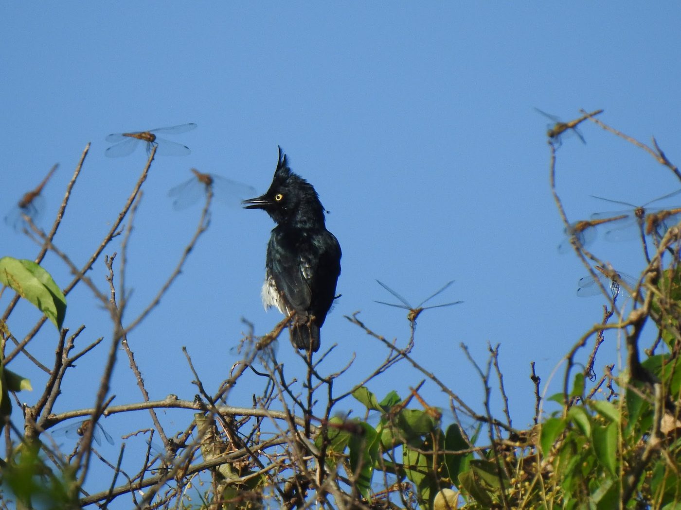
  <img src="/assets/writing/the-poisson-bootstrap/shrike-flycatcher.jpg" alt="A black-and-white shrike-flycatcher perched, with dragonflies" />
  <figcaption>Black-and-white shrike-flycatcher with <em>Trithemis</em> dragonflies, Entebbe</figcaption>
</figure>

<p>Bootstrapping is a useful technique to infer statistical features (think mean, decile, confidence intervals) of a population based on a sample collected. Implementing it at scale can be hard and in use cases with streaming data, very complicated. When trying to learn how to bootstrap at scale, I <a href="https://www.unofficialgoogledatascience.com/2015/08/an-introduction-to-poisson-bootstrap26.html">came across a Google blog</a> (almost a decade old) that introduces Poisson bootstrapping. Since then I’ve discovered an even older paper, <a href="http://www.med.mcgill.ca/epidemiology/Hanley/Reprints/bootstrap-hanley-macgibbon2006.pdf">Hanley and MacGibbon (2006)</a>, that outlines a version of this technique. This post is an attempt to make sure I’ve understood the logic well enough to explain it to someone else. We’ll start with a description of classical bootstrapping first to motivate why Poisson bootstrapping is neat.</p>

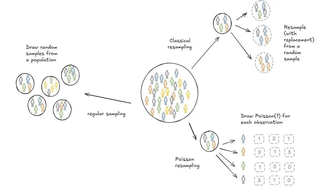
<p><img src="/assets/writing/the-poisson-bootstrap/repeated-sampling.png" alt="Drawing repeated samples from a population" /></p>

<h3 id="classical-bootstrapping">Classical bootstrapping</h3>

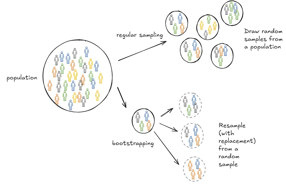
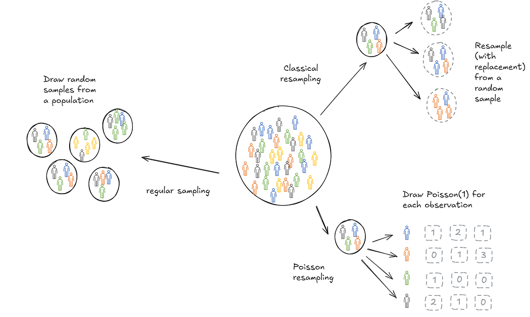
<p>Suppose we wanted to calculate the mean age of students in a school. We could repeatedly draw samples of 100 students, calculate the means and store them. Then we could take a final mean of those sample means. This final mean is an estimate of the population mean.</p>

<p>In practice, it’s often not possible to draw repeated samples from a population. This is where bootstrapping comes in. Bootstrapping sort of mimics this process. Instead of drawing samples from the population we draw samples (with replacement) from the one sample we collected. The psuedo-samples are referred to as resamples.</p>

<p><img src="/assets/writing/the-poisson-bootstrap/resampling.png" alt="Resampling with replacement from a single sample" /></p>

<p>Turns out this is extremely effective. It’s more computationally expensive than a closed form solution but does not make strong assumptions about the distribution of the population. Additionally, it’s cheaper than repeating sample collections. In practice, it’s used a lot in industry because in many cases either closed form solutions don’t exist or are hard to get right—for instance, when inferring deciles of a population.</p>

<h3 id="why-does-bootstrapping-work">Why does bootstrapping work?</h3>

<p>Bootstrapping feels wrong. Or at least the first time I learned about it, it didn’t feel right. Why should one sample contain so much information?</p>

<p>Sampling with replacement from the original sample you drew is just a way for you to mimic drawing from the population. The original sample you drew, on average, looks like your population. So when you resample from it, you’re essentially drawing samples from the same probability distribution.</p>

<p>What if you just happen to draw a weird sample? That’s possible and that’s why we resample. Resampling helps us learn about the distribution of the sample itself. What if you original sample is too small? As the number of observations in the sample grow, bootstrapping estimates converge to population values. However, there are no guarantees over finite samples.</p>

<p>There are problems but given the constraints we operate in, it is the best possible information we have on the population. We don’t have to assume the population has a specific shape. Given that computation is fairly cheap, bootstrapping becomes a very powerful tool to use.</p>

<h3 id="demonstrating-classical-bootstrapping">Demonstrating classical bootstrapping</h3>

<p>We’ll explain bootstrapping with two examples. The first is a tiny dataset where the idea is that you can do the math in your head. The second is a larger dataset for which I’ll write down code.</p>

<h3 id="example-1-determining-the-mean-age-of-students-in-a-school">Example 1: Determining the mean age of students in a school</h3>

<p>We’re tasked to determine the mean age of students in a school. We sample 5 students randomly. The idea is to use those 5 students to infer the average age of all the students in the school. This is silly (and statistically improper) but bear with me.</p>

<div class="language-python highlighter-rouge"><div class="highlight"><pre class="highlight"><code><span class="n">ages</span> <span class="o">=</span> <span class="p">[</span><span class="mi">12</span><span class="p">,</span> <span class="mi">8</span><span class="p">,</span> <span class="mi">10</span><span class="p">,</span> <span class="mi">15</span><span class="p">,</span> <span class="mi">9</span><span class="p">]</span>
</code></pre></div></div>

<p>We now sample from this list with replacement.</p>

<div class="language-python highlighter-rouge"><div class="highlight"><pre class="highlight"><code><span class="n">sample_1</span> <span class="o">=</span> <span class="p">[</span> <span class="mi">8</span><span class="p">,</span> <span class="mi">10</span><span class="p">,</span>  <span class="mi">8</span><span class="p">,</span> <span class="mi">15</span><span class="p">,</span> <span class="mi">12</span><span class="p">]</span>
<span class="n">sample_2</span> <span class="o">=</span> <span class="p">[</span><span class="mi">10</span><span class="p">,</span> <span class="mi">10</span><span class="p">,</span> <span class="mi">12</span><span class="p">,</span>  <span class="mi">8</span><span class="p">,</span> <span class="mi">15</span><span class="p">]</span>
<span class="n">sample_3</span> <span class="o">=</span> <span class="p">[</span><span class="mi">10</span><span class="p">,</span> <span class="mi">12</span><span class="p">,</span>  <span class="mi">9</span><span class="p">,</span>  <span class="mi">9</span><span class="p">,</span>  <span class="mi">9</span><span class="p">]</span>
<span class="p">....</span>
<span class="n">do</span> <span class="n">this</span> <span class="n">a</span> <span class="mi">1000</span> <span class="n">times</span>
<span class="p">....</span>
<span class="n">sample_1000</span> <span class="o">=</span> <span class="p">[</span> <span class="mi">9</span><span class="p">,</span> <span class="mi">12</span><span class="p">,</span> <span class="mi">12</span><span class="p">,</span> <span class="mi">15</span><span class="p">,</span>  <span class="mi">8</span><span class="p">]</span>
</code></pre></div></div>

<p>For each resample, calculate the mean.</p>

<div class="language-python highlighter-rouge"><div class="highlight"><pre class="highlight"><code><span class="n">mean_sample_1</span> <span class="o">=</span> <span class="mf">10.6</span>
<span class="n">mean_sample_2</span> <span class="o">=</span> <span class="mi">11</span>
<span class="n">mean_sample_3</span> <span class="o">=</span> <span class="mf">9.8</span>
<span class="p">...</span>
<span class="n">mean_sample_1000</span> <span class="o">=</span> <span class="mf">11.2</span>
</code></pre></div></div>

<p>Take a mean of those means.</p>

<div class="language-python highlighter-rouge"><div class="highlight"><pre class="highlight"><code><span class="n">mean_over_samples</span><span class="o">=</span><span class="n">mean</span><span class="p">(</span><span class="n">mean_sample_1</span><span class="p">,</span> <span class="n">mean_sample_2</span><span class="p">,</span> <span class="p">..</span> <span class="p">,</span> <span class="n">mean_sample_1000</span><span class="p">)</span>
</code></pre></div></div>

<p>This mean then becomes your estimate of the population mean. You can do the same thing over any statistical property: Confidence intervals, deviations etc.</p>

<h3 id="example-2-determining-the-95th-percentile-for-time-to-process-payment">Example 2: Determining the 95th percentile for ‘time to process payment’</h3>

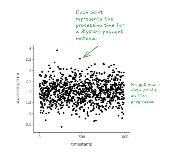
<p>Customers on a food delivery app make payments on the app. After a payment is successful, an order is placed with the restaurant. The <strong>time to process payment</strong> calculated as the time between when a customer presses the ‘Make Payment’ button and when feedback is delivered (payment successful, payment failed) is a critical metric that reflects platform reliability. Millions of customers make payments on the app every day.</p>

<p>We’re tasked to estimate the 95% percentile of the distribution to be able to rapidly detect issues.</p>

<p><img src="/assets/writing/the-poisson-bootstrap/payment-times.png" alt="Distribution of payment processing times" /></p>

<p>We illustrate classical bootstrapping in the following way:</p>

<ul>
  <li>We assume that there’s some population that has a million observations. In the real world, we never observe this data.</li>
  <li>We randomly sample 1/10th of this population. So we take 10,000 observations. In reality this is the only data we observe.</li>
  <li>We then apply the same procedure we discussed above. We resample observations from our observed data with replacement. We do this many, many times.</li>
  <li>Each time when we resample, we calculate the 95th percentile of that distribution.</li>
  <li>Finally we take the mean of the 95th percentile values and find confidence intervals around it.</li>
</ul>

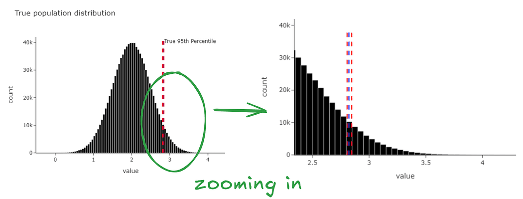
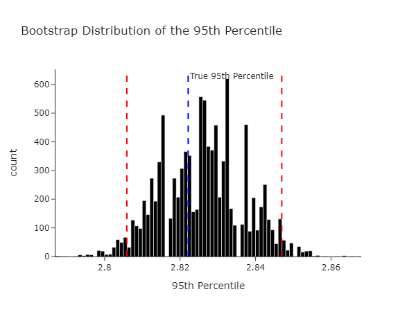
<p>We get the graph below. Magically, we find that the confidence intervals we just generated contain the true 95th percentile (from our population).</p>

<p><img src="/assets/writing/the-poisson-bootstrap/ci-contains-true.png" alt="Bootstrapped confidence intervals containing the true 95th percentile" /></p>

<p>We can see the same data at the level of the bootstrapped statistic.</p>

<p><img src="/assets/writing/the-poisson-bootstrap/bootstrapped-statistic.png" alt="The distribution of the bootstrapped statistic" /></p>

<p>The code to generate the above is below, give it a try yourself!</p>

<div class="language-python highlighter-rouge"><div class="highlight"><pre class="highlight"><code><span class="k">def</span> <span class="nf">bootstrap_nth_percentile_and_ci</span><span class="p">(</span>
    <span class="n">data</span><span class="p">:</span> <span class="n">List</span><span class="p">[</span><span class="nb">float</span><span class="p">],</span> <span class="n">n_iter</span><span class="p">:</span> <span class="nb">int</span> <span class="o">=</span> <span class="mi">1000</span><span class="p">,</span> <span class="n">alpha</span><span class="p">:</span> <span class="nb">float</span> <span class="o">=</span> <span class="mf">0.95</span><span class="p">,</span> <span class="n">percentile</span><span class="p">:</span> <span class="nb">float</span> <span class="o">=</span> <span class="mi">95</span>
<span class="p">)</span> <span class="o">-&gt;</span> <span class="n">Tuple</span><span class="p">[</span><span class="nb">float</span><span class="p">,</span> <span class="nb">float</span><span class="p">,</span> <span class="nb">float</span><span class="p">,</span> <span class="nb">float</span><span class="p">]:</span>
    <span class="s">"""Compute the nth percentile and confidence interval using bootstrapping

    Args:
        data (List[float]): List of data
        n_iter (int, optional): Number of bootstrap samples. Defaults to 1000.
        alpha (float, optional): Confidence level. Defaults to 0.95.
        percentile (float, optional): Percentile to compute. Defaults to 95.

    Returns:
        Tuple[float, float, float, float]: Tuple containing the percentile, mean,
        lower bound, and upper bound

    """</span>

    <span class="n">n</span> <span class="o">=</span> <span class="nb">len</span><span class="p">(</span><span class="n">data</span><span class="p">)</span>

    <span class="n">bootstrap_samples</span> <span class="o">=</span> <span class="n">np</span><span class="p">.</span><span class="n">random</span><span class="p">.</span><span class="n">choice</span><span class="p">(</span><span class="n">data</span><span class="p">,</span> <span class="p">(</span><span class="n">n_iter</span><span class="p">,</span> <span class="n">n</span><span class="p">),</span> <span class="n">replace</span><span class="o">=</span><span class="bp">True</span><span class="p">)</span>
    <span class="n">percentiles</span> <span class="o">=</span> <span class="n">np</span><span class="p">.</span><span class="n">percentile</span><span class="p">(</span><span class="n">bootstrap_samples</span><span class="p">,</span> <span class="n">percentile</span><span class="p">,</span> <span class="n">axis</span><span class="o">=</span><span class="mi">1</span><span class="p">)</span>

    <span class="n">mean</span> <span class="o">=</span> <span class="n">percentiles</span><span class="p">.</span><span class="n">mean</span><span class="p">()</span>
    <span class="n">lower</span> <span class="o">=</span> <span class="n">np</span><span class="p">.</span><span class="n">percentile</span><span class="p">(</span><span class="n">percentiles</span><span class="p">,</span> <span class="p">(</span><span class="mi">1</span> <span class="o">-</span> <span class="n">alpha</span><span class="p">)</span> <span class="o">/</span> <span class="mi">2</span> <span class="o">*</span> <span class="mi">100</span><span class="p">)</span>
    <span class="n">upper</span> <span class="o">=</span> <span class="n">np</span><span class="p">.</span><span class="n">percentile</span><span class="p">(</span><span class="n">percentiles</span><span class="p">,</span> <span class="p">(</span><span class="mi">1</span> <span class="o">+</span> <span class="n">alpha</span><span class="p">)</span> <span class="o">/</span> <span class="mi">2</span> <span class="o">*</span> <span class="mi">100</span><span class="p">)</span>

    <span class="k">return</span> <span class="n">percentiles</span><span class="p">,</span> <span class="n">mean</span><span class="p">,</span> <span class="n">lower</span><span class="p">,</span> <span class="n">upper</span>


<span class="c1"># population specifics
</span><span class="n">mean_time</span> <span class="o">=</span> <span class="mf">2.0</span>
<span class="n">std_dev</span> <span class="o">=</span> <span class="mf">0.5</span>
<span class="n">processing_time</span> <span class="o">=</span> <span class="n">np</span><span class="p">.</span><span class="n">random</span><span class="p">.</span><span class="n">normal</span><span class="p">(</span><span class="n">loc</span><span class="o">=</span><span class="n">mean_time</span><span class="p">,</span> <span class="n">scale</span><span class="o">=</span><span class="n">std_dev</span><span class="p">,</span> <span class="n">size</span><span class="o">=</span><span class="mi">1_000_000</span><span class="p">)</span>

<span class="c1"># sample from processing time
</span><span class="n">sample</span> <span class="o">=</span> <span class="n">np</span><span class="p">.</span><span class="n">random</span><span class="p">.</span><span class="n">choice</span><span class="p">(</span><span class="n">processing_time</span><span class="p">,</span> <span class="mi">10000</span><span class="p">)</span> <span class="c1"># note we only sample 1/10th of the population
</span>
<span class="n">percentiles</span><span class="p">,</span> <span class="n">mean</span><span class="p">,</span> <span class="n">lower_bound</span><span class="p">,</span> <span class="n">upper_bound</span> <span class="o">=</span> <span class="n">bootstrap_nth_percentile_and_ci</span><span class="p">(</span>
    <span class="n">sample</span><span class="p">,</span> <span class="n">n_iter</span><span class="o">=</span><span class="mi">10000</span><span class="p">,</span> <span class="n">percentile</span><span class="o">=</span><span class="mi">95</span>
<span class="p">)</span>
</code></pre></div></div>

<h2 id="this-all-works-great-whats-next">This all works great, what’s next?</h2>

<p>Now that we’ve established that classical bootstrapping actually works we’ll try and establish what’s happening from a mathematical perspective. Usually texts will just tell you to skip this part if you’re not interested. I’ll encourage you to stick around though because this is where the real fun is.</p>

<h3 id="take-a-break">Take a break</h3>

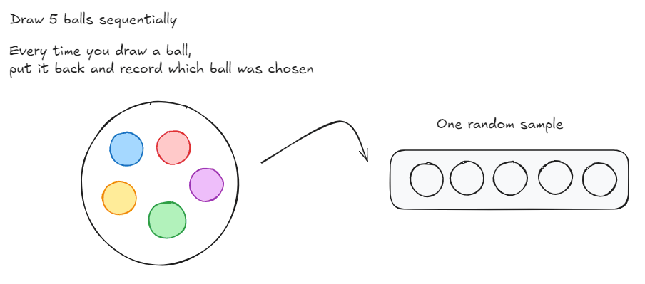
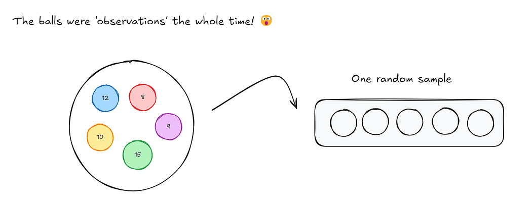
<p>Let’s think through a game now. Imagine you had a bag filled with 5 balls: A red, blue, yellow, green and purple ball. You need to draw 5 balls from the bag, one at a time. After you draw a ball, you put it back into the bag and then draw again. So each time you choose a ball, you have 5 differently coloured balls to choose from. After each round you record the ball that was chosen in a empty slot (as shown below).</p>

<p><img src="/assets/writing/the-poisson-bootstrap/balls-and-slots.png" alt="Five coloured balls and five slots to fill" /></p>

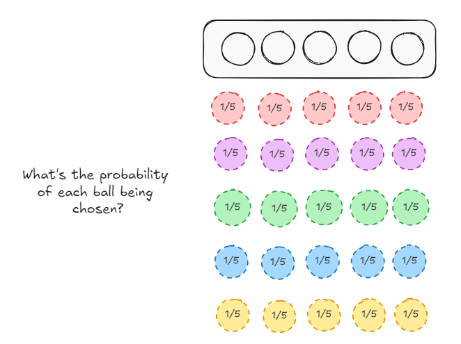
<p>Now, if I were to ask you, what’s the probability of each ball being chosen for a each slot that we have to fill?</p>

<p>For slot 1,</p>

<ul>
  <li>The red ball can be chosen with probability 1/5</li>
  <li>The purple ball can be chosen with probability 1/5</li>
  <li>The green ball can be chosen with probability 1/5</li>
  <li>The blue ball can be chosen with probability 1/5</li>
  <li>The yellow ball can be chosen with probability 1/5</li>
</ul>

<p>The same case extends to slot 2, 3, 4 and 5</p>

<p><img src="/assets/writing/the-poisson-bootstrap/slot-probabilities.png" alt="The same probabilities across every slot" /></p>

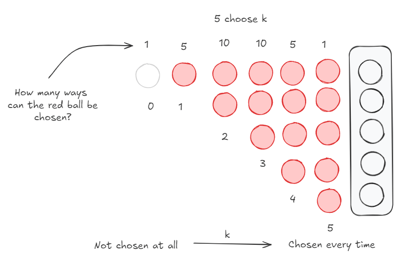
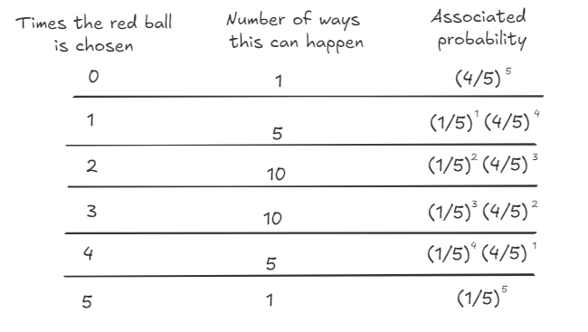
<p>Lets focus on the red ball for a bit. It can be chosen a minimum of zero times (it isn’t chosen at all) and a maximum of 5 times. The probability distribution of the occurrence of the red ball is the following:</p>

<ul>
  <li>Red ball chosen 0 times: This can only happen in 1 way.</li>
  <li>Red ball chosen 1 time: This can happen in 5 ways. Red ball is chosen for slot 1, Red ball is chosen for slot 2 … (you get the drift).</li>
  <li>Red ball chosen 2 times: This can happen in 10 ways. Fix the red ball on slot 1, there are 4 options. Fix the red ball on slot 2, there are 3 new options, …</li>
  <li>Red ball chosen 3 times: This can happen in 10 ways. This is exactly similar to the logic above.</li>
  <li>Red ball chosen 4 times: The can happen in 5 ways. Similar to being chosen once.</li>
  <li>Red ball is chosen 5 times. This can happen in 1 way.</li>
</ul>

<p>This is just <em>5 choose k</em>, where <em>k = {0, 1, 2, 3, 4, 5}</em></p>

<p><img src="/assets/writing/the-poisson-bootstrap/n-choose-k.png" alt="5 choose k for k from zero to five" /></p>

<p>Let’s put these two facts together just for the red balls</p>

<p><img src="/assets/writing/the-poisson-bootstrap/red-ball-distribution.png" alt="Combining the counts and the probabilities for the red ball" /></p>

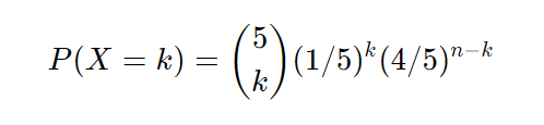
<p>What we just described is the binomial distribution where <em>n = 5</em> and <em>p = 1/5</em></p>

<p><img src="/assets/writing/the-poisson-bootstrap/binomial-n5.png" alt="The binomial distribution with n equals five and p equals one fifth" /></p>

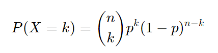
<p>Or more generally,</p>

<p><img src="/assets/writing/the-poisson-bootstrap/binomial-general.png" alt="The general form of the binomial distribution" /></p>

<p>Now just substitute balls for observations.</p>

<p><img src="/assets/writing/the-poisson-bootstrap/binomial-observations.png" alt="The same distribution applied to observations rather than balls" /></p>

<p>So when we bootstrap, we essentially are drawing each observation from a binomial distribution.</p>

<blockquote>
  <p>In classical bootstrapping, when we resample, each observation follows the binomial distribution with n = n, k = {0, …, n} and p = 1/n. This is also expressed as Binomial(n , 1/n).</p>
</blockquote>

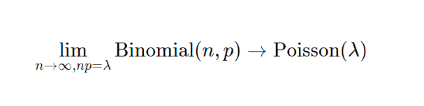
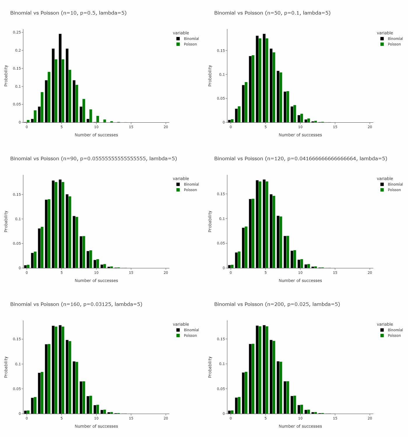
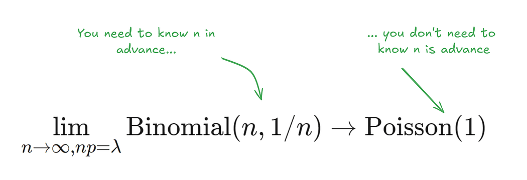
<p>Now, a very interesting property of the binomial distribution is that as n turns larger and larger, and p turns smaller and smaller, the binomial distribution converges to a Poisson distribution with <em>Poisson(n/p)</em>. Some day I’ll write an intuitive explanation of why this happens but for now if you’re interested, you can read <a href="https://medium.com/@andrew.chamberlain/deriving-the-poisson-distribution-from-the-binomial-distribution-840cc1668239">this very well written piece</a>.</p>

<p><img src="/assets/writing/the-poisson-bootstrap/binomial-to-poisson.png" alt="The binomial converging to the Poisson" /></p>

<p>This works for any n and p such that n/p is constant. In the gif below we show this for lambda (n/p) = 5.</p>

<p><img src="/assets/writing/the-poisson-bootstrap/lambda-5.gif" alt="Animation of the convergence for lambda equals five" /></p>

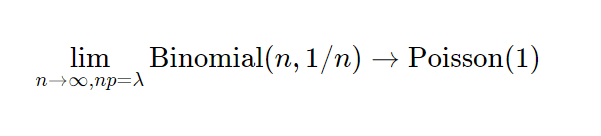
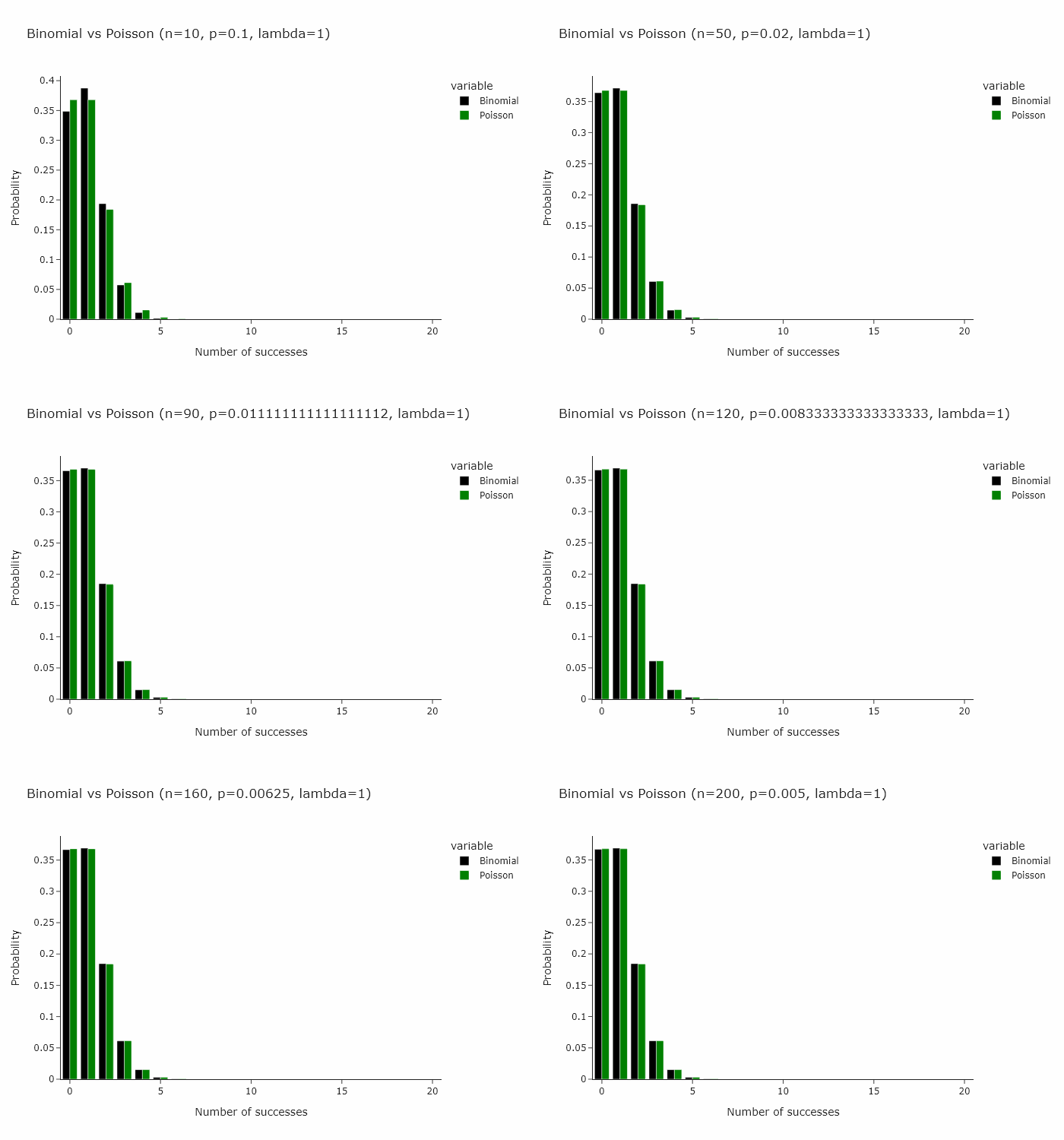
<p>In our special case, we’ll just converge to <em>Poisson(1)</em> as p is just 1/n.</p>

<p><img src="/assets/writing/the-poisson-bootstrap/poisson-1.png" alt="Convergence to Poisson of one" /></p>

<p><img src="/assets/writing/the-poisson-bootstrap/poisson-convergence.gif" alt="Animation of the convergence to Poisson of one" /></p>

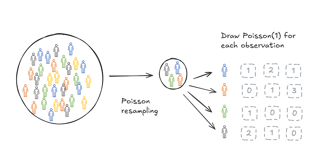
<p>Then it follow that another way to resample would be to draw each observation from a Poisson(1) distribution.</p>

<blockquote class="note">
  <p>Poisson bootstrapping means that we use a Poisson(1) process to generate resamples for bootstrapping a statistic.</p>
</blockquote>

<p><img src="/assets/writing/the-poisson-bootstrap/poisson-resamples.png" alt="Generating resamples with a Poisson process" /></p>

<h2 id="big-deal-why-is-this-useful">Big deal, why is this useful?</h2>

<p>There are two stages of bootstrapping a statistic of interest. The first stage is to create resamples, the second stage is to calculate the statistic on each resample. Classical and Poisson bootstrapping are identical on the second stage but different on the first stage.</p>

<p>There are two ways in which this is useful:</p>

<ul>
  <li>Poisson bootstrapping reduces the number of passes we need to make over data.</li>
  <li>Poisson bootstrapping works in cases where we don’t have a fixed n. For instance, when we’re streaming data in.</li>
</ul>

<h3 id="reducing-the-number-of-passes-while-resampling">Reducing the number of passes while resampling</h3>

<p>The Poisson bootstrap allows for significant computation gains while creating resamples. The best way to look at this is in code.</p>

<div class="language-python highlighter-rouge"><div class="highlight"><pre class="highlight"><code><span class="k">def</span> <span class="nf">poisson_bootstrap_nth_percentile_and_ci</span><span class="p">(</span>
    <span class="n">data</span><span class="p">:</span> <span class="n">List</span><span class="p">[</span><span class="nb">float</span><span class="p">],</span> <span class="n">n_iter</span><span class="p">:</span> <span class="nb">int</span> <span class="o">=</span> <span class="mi">1000</span><span class="p">,</span> <span class="n">alpha</span><span class="p">:</span> <span class="nb">float</span> <span class="o">=</span> <span class="mf">0.95</span><span class="p">,</span> <span class="n">percentile</span><span class="p">:</span> <span class="nb">float</span> <span class="o">=</span> <span class="mi">95</span>
<span class="p">)</span> <span class="o">-&gt;</span> <span class="n">Tuple</span><span class="p">[</span><span class="nb">float</span><span class="p">,</span> <span class="nb">float</span><span class="p">,</span> <span class="nb">float</span><span class="p">,</span> <span class="nb">float</span><span class="p">]:</span>

    <span class="n">data</span> <span class="o">=</span> <span class="n">np</span><span class="p">.</span><span class="n">array</span><span class="p">(</span><span class="n">data</span><span class="p">)</span>
    <span class="n">n</span> <span class="o">=</span> <span class="nb">len</span><span class="p">(</span><span class="n">data</span><span class="p">)</span>

    <span class="n">weights</span> <span class="o">=</span> <span class="n">np</span><span class="p">.</span><span class="n">random</span><span class="p">.</span><span class="n">poisson</span><span class="p">(</span><span class="mi">1</span><span class="p">,</span> <span class="p">(</span><span class="n">n_iter</span><span class="p">,</span> <span class="n">n</span><span class="p">))</span>

    <span class="n">percentiles</span> <span class="o">=</span> <span class="p">[]</span>

    <span class="k">for</span> <span class="n">weight</span> <span class="ow">in</span> <span class="n">weights</span><span class="p">:</span>
        <span class="n">resampled_data</span> <span class="o">=</span> <span class="n">np</span><span class="p">.</span><span class="n">repeat</span><span class="p">(</span><span class="n">data</span><span class="p">,</span> <span class="n">weight</span><span class="p">)</span>
        <span class="n">percentile</span> <span class="o">=</span> <span class="n">np</span><span class="p">.</span><span class="n">percentile</span><span class="p">(</span><span class="n">resampled_data</span><span class="p">,</span> <span class="mi">95</span><span class="p">)</span>
        <span class="n">percentiles</span><span class="p">.</span><span class="n">append</span><span class="p">(</span><span class="n">percentile</span><span class="p">)</span>

    <span class="n">mean_percentile</span> <span class="o">=</span> <span class="n">np</span><span class="p">.</span><span class="n">mean</span><span class="p">(</span><span class="n">percentiles</span><span class="p">)</span>
    <span class="n">lower_bound</span> <span class="o">=</span> <span class="n">np</span><span class="p">.</span><span class="n">percentile</span><span class="p">(</span><span class="n">percentiles</span><span class="p">,</span> <span class="p">(</span><span class="mi">1</span> <span class="o">-</span> <span class="n">alpha</span><span class="p">)</span> <span class="o">/</span> <span class="mi">2</span> <span class="o">*</span> <span class="mi">100</span><span class="p">)</span>
    <span class="n">upper_bound</span> <span class="o">=</span> <span class="n">np</span><span class="p">.</span><span class="n">percentile</span><span class="p">(</span><span class="n">percentiles</span><span class="p">,</span> <span class="p">(</span><span class="mi">1</span> <span class="o">+</span> <span class="n">alpha</span><span class="p">)</span> <span class="o">/</span> <span class="mi">2</span> <span class="o">*</span> <span class="mi">100</span><span class="p">)</span>

    <span class="k">return</span> <span class="n">percentiles</span><span class="p">,</span> <span class="n">mean_percentile</span><span class="p">,</span> <span class="n">lower_bound</span><span class="p">,</span> <span class="n">upper_bound</span>
</code></pre></div></div>

<p>Compare line (8) above, with the equivalent line in the classical bootstrap:</p>

<div class="language-python highlighter-rouge"><div class="highlight"><pre class="highlight"><code><span class="c1"># classical, needs to know (data)
</span><span class="n">bootstrap_samples</span> <span class="o">=</span> <span class="n">np</span><span class="p">.</span><span class="n">random</span><span class="p">.</span><span class="n">choice</span><span class="p">(</span><span class="n">data</span><span class="p">,</span> <span class="p">(</span><span class="n">n_iter</span><span class="p">,</span> <span class="n">n</span><span class="p">),</span> <span class="n">replace</span><span class="o">=</span><span class="bp">True</span><span class="p">)</span>

<span class="c1"># poisson, does not need to know (data)
</span><span class="n">weights</span> <span class="o">=</span> <span class="n">np</span><span class="p">.</span><span class="n">random</span><span class="p">.</span><span class="n">poisson</span><span class="p">(</span><span class="mi">1</span><span class="p">,</span> <span class="p">(</span><span class="n">n_iter</span><span class="p">,</span> <span class="n">n</span><span class="p">))</span>
</code></pre></div></div>

<p>In the classical bootstrap, you need to know <em>data</em>, while in the Poisson bootstrap you don’t.</p>

<p>The implications for this are very significant for cases where data is very large (think 100s of millions of observations). This is because mathematically, generating resamples reduces to generating counts for each observation.</p>

<ul>
  <li>In classical bootstrapping, the counts for each observation follow a <em>Binomial(n, 1/n)</em>. Together they follow a <a href="https://en.wikipedia.org/wiki/Multinomial_distribution"><em>Multinomial(n, 1/n, 1/n, …, 1/n)</em></a>. This means when you generate a count for an observation, this impacts the count for the other observations. For instance, in our ball example, once you’ve generated the count for a red ball, this has a direct impact on the counts for the other balls. For instance, if the count for the red ball is 2, then we know that we only have 3 more balls we can choose.</li>
  <li>In Poisson bootstrapping, the counts for each observation are independent on each other. So if you need 1000 resamples, you just generate 1000 Poisson(1) draws for the red ball. Then you’re done and you can move on to the next observation.</li>
</ul>

<h3 id="resampling-when-n-is-unknown">Resampling when n is unknown</h3>

<p>There are cases where n is effectively unknown. For instance, in cases where you’re streaming in payment data or where data is so large that is lives across multiple storage instances.</p>

<p><img src="/assets/writing/the-poisson-bootstrap/streaming.png" alt="Resampling over streaming data" /></p>

<p>In classical bootstrapping every time we observe an increased n, we have to redo the resampling process again (as we sample with replacement). This renders this method quite computationally expensive and wasteful. In the Poisson bootstrap we can just save our <em>Poisson(1)</em> draws for each instance. Every time a new instance is added all we need to do is to generate the <em>Poisson(1)</em> draws for this new instance.</p>

<h2 id="conclusion">Conclusion</h2>

<p><img src="/assets/writing/the-poisson-bootstrap/conclusion.png" alt="Classical and Poisson bootstrapping side by side" /></p>

<p>Classical bootstrapping is a very effective technique for learning the distribution of a statistic from a sample collected. In practice, it can be prohibitively expensive for very large datasets. Poisson bootstrapping is a version of bootstrapping that enables efficient parallel computation of resamples. This is because of two reasons:</p>

<ol>
  <li>Resampling under Poisson bootstraps means we only make one pass over each observation.</li>
  <li>In streaming data cases, Poisson bootstraps allow us to process new resamples incrementally rather than having to resample over the entire dataset in one go.</li>
</ol>]]></content><author><name>David Clarance</name></author><category term="A/B Testing" /><category term="Bootstrapping" /><summary type="html"><![CDATA[Black-and-white shrike-flycatcher with Trithemis dragonflies, Entebbe]]></summary></entry><entry><title type="html">Stable and fast randomization using hash spaces</title><link href="https://davidclarance.github.io/writing/stable-and-fast-randomization-using-hash-spaces/" rel="alternate" type="text/html" title="Stable and fast randomization using hash spaces" /><published>2024-06-29T00:00:00+00:00</published><updated>2024-06-29T00:00:00+00:00</updated><id>https://davidclarance.github.io/writing/stable-and-fast-randomization-using-hash-spaces</id><content type="html" xml:base="https://davidclarance.github.io/writing/stable-and-fast-randomization-using-hash-spaces/"><![CDATA[<figure>
  <img src="/assets/writing/stable-and-fast-randomization-using-hash-spaces/mountain-wagtail.jpg" alt="A mountain wagtail on a rock" />
  <figcaption>Mountain Wagtail, Karura Forest</figcaption>
</figure>

<p>A core part of running an experiment is to assign an experimental unit (for instance a customer) to a specific treatment (payment button variant, marketing push notification framing). Often this assignment needs to meet the following conditions:</p>

<ol>
  <li>It needs to be random.</li>
  <li>It needs to be stable. If the customer comes back to the screen, they need to be exposed to the same payment button variant.</li>
  <li>It needs to be retrieved or generated very quickly.</li>
  <li>It needs to be available after the actual assignment so it can be used in downstream analysis.</li>
</ol>

<p>When organizations first start their experimentation journey, a common pattern is to pre-generate assignments, store it in a database and then retrieve it at the time of assignment. This is a perfectly valid method to use and works great when you’re starting off. However, as you start to scale in customer and experiment volumes, this method becomes harder and harder to maintain and use reliably. You’ve got to (a) manage the complexity of storage, (b) ensure that assignments are actually random <em>within</em> and <em>across</em> experiments, and (c) retrieve the assignment reliably. All of these are hard at scale.</p>

<p>Using <em>hash spaces</em> helps solve some of these problems. It’s a simple solution but isn’t as widely known as it probably should be. This blog is an attempt to explain the technique. There are links to code in different languages at the end. However, if you’d like, you can also directly <a href="https://gist.github.com/davidclarance/daeafad5fc3e28e019950a12b0da01f5">jump to code here</a>.</p>

<figure>
  <img src="/assets/writing/stable-and-fast-randomization-using-hash-spaces/solution-overview.png" alt="Diagram of the hash space approach end to end" />
  <figcaption>An overview of the solution</figcaption>
</figure>

<h2 id="setting-up">Setting up</h2>

<p>We’re running an experiment to test which variant of a progress bar on our customer app drives the most engagement. There are three variants: Control (the default experience), Variant A and Variant B.</p>

<p>We have 10 million customers that use our app every week and we want to ensure that these 10 million customers get randomly assigned to one of the three variants. Each time the customer comes back to the app they should see the same variant. We want control to be assigned with a 50% probability, Variant 1 to be assigned with a 30% probability and Variant 2 to be assigned with a 20% probability.</p>

<div class="language-python highlighter-rouge"><div class="highlight"><pre class="highlight"><code><span class="n">probability_assignments</span> <span class="o">=</span> <span class="p">{</span><span class="s">"Control"</span><span class="p">:</span> <span class="mi">50</span><span class="p">,</span> <span class="s">"Variant 1"</span><span class="p">:</span> <span class="mi">30</span><span class="p">,</span> <span class="s">"Variant 2"</span><span class="p">:</span> <span class="mi">20</span><span class="p">}</span>
</code></pre></div></div>

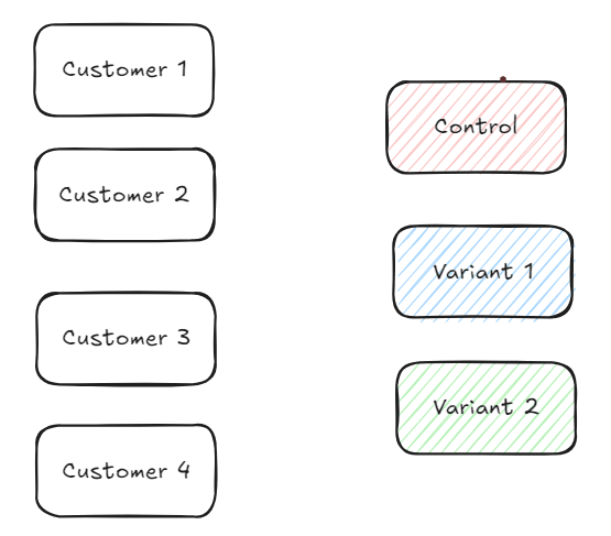
<p>To make things simpler, we’ll start with 4 customers. These customers have IDs that we use to refer to them. These IDs are generally either GUIDs (something like <code class="language-plaintext highlighter-rouge">"b7be65e3-c616-4a56-b90a-e546728a6640"</code>) or integers (like 1019222, 1028333). Any of these ID types would work but to make things easier to follow we’ll simply assume that these IDs are: “Customer1”, “Customer2”, “Customer3”, “Customer4”.</p>

<p><img src="/assets/writing/stable-and-fast-randomization-using-hash-spaces/four-customers.png" alt="Four customers to be assigned to variants" /></p>

<p>Our goal is to map these 4 customers to the three possible variants.</p>

<h2 id="hashing-customer-ids">Hashing customer IDs</h2>

<p>This method primarily relies on using hash algorithms that come with some very desirable properties. Hashing algorithms take a string of arbitrary length and map it to a ‘hash’ of a fixed length. The easiest way to understand this is through some examples.</p>

<p>A hash function, takes a string and maps it to a constant hash space. In the example below, a hash function (in this case <a href="https://en.wikipedia.org/wiki/MD5">md5</a>) takes the words: “Hello”, “World”, “Hello World” and “Hello WorLd” (note the capital L) and maps it to an alphanumeric string of 32 characters.</p>

<p><img src="/assets/writing/stable-and-fast-randomization-using-hash-spaces/md5-examples.png" alt="md5 hashes of four similar strings" /></p>

<p>A few important things to note:</p>

<ul>
  <li>The hashes are all of the same length.</li>
  <li>A minor difference in the input (capital L instead of small L) changes the hash.</li>
  <li>Hashes are a hexadecimal string. That is, they comprise of the numbers 0 to 9 and the first six alphabets (a, b, c, d, e and f).</li>
</ul>

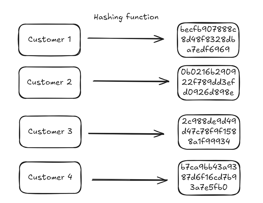
<p>We can use this same logic and get hashes for our four customers:</p>

<div class="language-python highlighter-rouge"><div class="highlight"><pre class="highlight"><code><span class="kn">import</span> <span class="nn">hashlib</span>

<span class="n">representative_customers</span> <span class="o">=</span> <span class="p">[</span><span class="s">"Customer1"</span><span class="p">,</span> <span class="s">"Customer2"</span><span class="p">,</span> <span class="s">"Customer3"</span><span class="p">,</span> <span class="s">"Customer4"</span><span class="p">]</span>

<span class="k">def</span> <span class="nf">get_hash</span><span class="p">(</span><span class="n">customer_id</span><span class="p">):</span>
    <span class="n">hash_object</span> <span class="o">=</span> <span class="n">hashlib</span><span class="p">.</span><span class="n">md5</span><span class="p">(</span><span class="n">customer_id</span><span class="p">.</span><span class="n">encode</span><span class="p">())</span>
    <span class="k">return</span> <span class="n">hash_object</span><span class="p">.</span><span class="n">hexdigest</span><span class="p">()</span>

<span class="p">{</span><span class="n">customer</span><span class="p">:</span> <span class="n">get_hash</span><span class="p">(</span><span class="n">customer</span><span class="p">)</span> <span class="k">for</span> <span class="n">customer</span> <span class="ow">in</span> <span class="n">representative_customers</span><span class="p">}</span>

<span class="c1"># {'Customer1': 'becfb907888c8d48f8328dba7edf6969',
#  'Customer2': '0b0216b290922f789dd3efd0926d898e',
#  'Customer3': '2c988de9d49d47c78f9f1588a1f99934',
#  'Customer4': 'b7ca9bb43a9387d6f16cd7b93a7e5fb0'}
</span></code></pre></div></div>

<p><img src="/assets/writing/stable-and-fast-randomization-using-hash-spaces/customer-hashes.png" alt="The four customer IDs and their hashes" /></p>

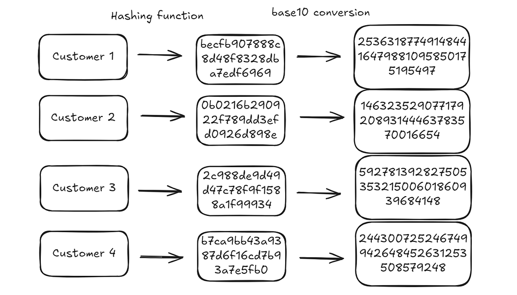
<p>Hexadecimal strings are just representations of numbers in base 16. We can <a href="https://g.co/gemini/share/83e1757e48f9">convert them to integers in base 10</a>.</p>

<blockquote class="note">
  <p>⚠️ One important note here: We rarely need to use the full hash. In practice (for instance in the linked code) we use a much smaller part of the hash (first 10 characters). Here we use the full hash to make explanations a bit easier.</p>
</blockquote>

<div class="language-python highlighter-rouge"><div class="highlight"><pre class="highlight"><code><span class="k">def</span> <span class="nf">get_integer_representation_of_hash</span><span class="p">(</span><span class="n">customer_id</span><span class="p">):</span>
    <span class="n">hash_value</span> <span class="o">=</span> <span class="n">get_hash</span><span class="p">(</span><span class="n">customer_id</span><span class="p">)</span>
    <span class="k">return</span> <span class="nb">int</span><span class="p">(</span><span class="n">hash_value</span><span class="p">,</span> <span class="mi">16</span><span class="p">)</span>

<span class="p">{</span>
    <span class="n">customer</span><span class="p">:</span> <span class="n">get_integer_representation_of_hash</span><span class="p">(</span><span class="n">customer</span><span class="p">)</span>
    <span class="k">for</span> <span class="n">customer</span> <span class="ow">in</span> <span class="n">representative_customers</span>
<span class="p">}</span>

<span class="c1"># {'Customer1': 253631877491484416479881095850175195497,
#  'Customer2': 14632352907717920893144463783570016654,
#  'Customer3': 59278139282750535321500601860939684148,
#  'Customer4': 244300725246749942648452631253508579248}
</span></code></pre></div></div>

<p><img src="/assets/writing/stable-and-fast-randomization-using-hash-spaces/hash-integers.png" alt="The hashes converted to base ten integers" /></p>

<p>There are two important properties of these integers:</p>

<ol>
  <li>These integers are <strong>stable</strong>: Given a fixed input (“Customer1”), the hashing algorithm will always give the same output.</li>
  <li>These integers are <strong>uniformly distributed</strong>: This one hasn’t been explained yet and mostly applies to cryptographic hash functions (such as md5). Uniformity is a design requirement for these hash functions. If they were not uniformly distributed, the chances of collisions (getting the same output for different inputs) would be higher and weaken the security of the hash. There are some <a href="https://www.rolando.cl/blog/2018/12/how_uniform_is_md5.html">explorations</a> of the <a href="https://stackoverflow.com/a/9346575/4583536">uniformity</a> property.</li>
</ol>

<p>Now that we have an integer representation of each ID that’s stable (always has the same value) and <a href="https://en.wikipedia.org/wiki/Hash_function#Uniformity">uniformly distributed</a>, we can use it to get to an assignment.</p>

<h2 id="from-integer-representations-to-assignment">From integer representations to assignment</h2>

<p>Going back to our probability assignments, we want to assign customers to variants with the following distribution:</p>

<div class="language-python highlighter-rouge"><div class="highlight"><pre class="highlight"><code><span class="p">{</span><span class="s">"Control"</span><span class="p">:</span> <span class="mi">50</span><span class="p">,</span> <span class="s">"Variant 1"</span><span class="p">:</span> <span class="mi">30</span><span class="p">,</span> <span class="s">"Variant 2"</span><span class="p">:</span> <span class="mi">20</span><span class="p">}</span>
</code></pre></div></div>

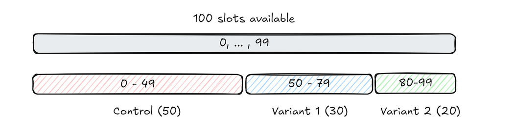
<p>If we had 100 slots, we can divide them into 3 buckets where the number of slots represents the probability we want to assign to that bucket. For instance, in our example, we divide the integer range 0–99 (100 units), into 0–49 (50 units), 50–79 (30 units) and 80–99 (20 units).</p>

<p><img src="/assets/writing/stable-and-fast-randomization-using-hash-spaces/partitions.png" alt="One hundred slots divided into three partitions" /></p>

<div class="language-python highlighter-rouge"><div class="highlight"><pre class="highlight"><code><span class="k">def</span> <span class="nf">divide_space_into_partitions</span><span class="p">(</span><span class="n">prob_distribution</span><span class="p">):</span>
    <span class="n">partition_ranges</span> <span class="o">=</span> <span class="p">[]</span>
    <span class="n">start</span> <span class="o">=</span> <span class="mi">0</span>
    <span class="k">for</span> <span class="n">partition</span> <span class="ow">in</span> <span class="n">prob_distribution</span><span class="p">:</span>
        <span class="n">partition_ranges</span><span class="p">.</span><span class="n">append</span><span class="p">((</span><span class="n">start</span><span class="p">,</span> <span class="n">start</span> <span class="o">+</span> <span class="n">partition</span><span class="p">))</span>
        <span class="n">start</span> <span class="o">+=</span> <span class="n">partition</span>
    <span class="k">return</span> <span class="n">partition_ranges</span>

<span class="n">divide_space_into_partitions</span><span class="p">(</span><span class="n">prob_distribution</span><span class="o">=</span><span class="n">probability_assignments</span><span class="p">.</span><span class="n">values</span><span class="p">())</span>

<span class="c1"># note that this is zero indexed, lower bound inclusive and upper bound exclusive
# [(0, 50), (50, 80), (80, 100)]
</span></code></pre></div></div>

<p>Now, if we assign a customer to one of the 100 slots randomly, the resultant distribution should then be equal to our intended distribution. Another way to think about this is, if we choose a number randomly between 0 and 99, there’s a 50% chance it’ll be between 0 and 49, 30% chance it’ll be between 50 and 79 and 20% chance it’ll be between 80 and 99.</p>

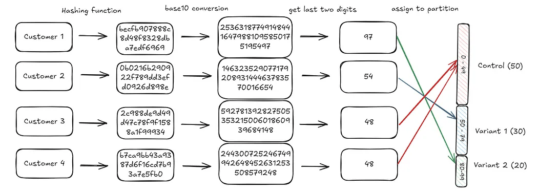
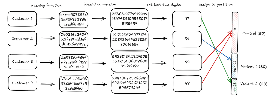
<p>The only remaining step is to map the customer integers we generated to one of these hundred slots. We do this by extracting the last two digits of the integer generated and using that as the assignment. For instance, the last two digits for customer 1 are 97 (you can check the diagram below). This falls in the third bucket (Variant 2) and hence the customer is assigned to Variant 2.</p>

<p>We repeat this process iteratively for each customer. When we’re done with all our customers, we should find that the end distribution will be what we’d expect: 50% of customers are in control, 30% in variant 1, 20% in variant 2.</p>

<div class="language-python highlighter-rouge"><div class="highlight"><pre class="highlight"><code><span class="k">def</span> <span class="nf">assign_groups</span><span class="p">(</span><span class="n">customer_id</span><span class="p">,</span> <span class="n">partitions</span><span class="p">):</span>
    <span class="n">hash_value</span> <span class="o">=</span> <span class="n">get_relevant_place_value</span><span class="p">(</span><span class="n">customer_id</span><span class="p">,</span> <span class="mi">100</span><span class="p">)</span>
    <span class="k">for</span> <span class="n">idx</span><span class="p">,</span> <span class="p">(</span><span class="n">start</span><span class="p">,</span> <span class="n">end</span><span class="p">)</span> <span class="ow">in</span> <span class="nb">enumerate</span><span class="p">(</span><span class="n">partitions</span><span class="p">):</span>
        <span class="k">if</span> <span class="n">start</span> <span class="o">&lt;=</span> <span class="n">hash_value</span> <span class="o">&lt;</span> <span class="n">end</span><span class="p">:</span>
            <span class="k">return</span> <span class="n">idx</span>
    <span class="k">return</span> <span class="bp">None</span>


<span class="n">partitions</span> <span class="o">=</span> <span class="n">divide_space_into_partitions</span><span class="p">(</span>
    <span class="n">prob_distribution</span><span class="o">=</span><span class="n">probability_assignments</span><span class="p">.</span><span class="n">values</span><span class="p">()</span>
<span class="p">)</span>

<span class="n">groups</span> <span class="o">=</span> <span class="p">{</span>
    <span class="n">customer</span><span class="p">:</span> <span class="nb">list</span><span class="p">(</span><span class="n">probability_assignments</span><span class="p">.</span><span class="n">keys</span><span class="p">())[</span><span class="n">assign_groups</span><span class="p">(</span><span class="n">customer</span><span class="p">,</span> <span class="n">partitions</span><span class="p">)]</span>
    <span class="k">for</span> <span class="n">customer</span> <span class="ow">in</span> <span class="n">representative_customers</span>
<span class="p">}</span>

<span class="c1"># output
# {'Customer1': 'Variant 2',
#  'Customer2': 'Variant 1',
#  'Customer3': 'Control',
#  'Customer4': 'Control'}
</span></code></pre></div></div>

<p>The <a href="https://gist.github.com/davidclarance/daeafad5fc3e28e019950a12b0da01f5?permalink_comment_id=5136729#gistcomment-5136729">linked gist</a> has a replication of the above for 1,000,000 customers where we can observe that customers are distributed in the expected proportions.</p>

<div class="language-python highlighter-rouge"><div class="highlight"><pre class="highlight"><code><span class="c1"># resulting proportions from a simulation on 1 million customers.
</span><span class="p">{</span><span class="s">'Variant 1'</span><span class="p">:</span> <span class="mf">0.299799</span><span class="p">,</span> <span class="s">'Variant 2'</span><span class="p">:</span> <span class="mf">0.199512</span><span class="p">,</span> <span class="s">'Control'</span><span class="p">:</span> <span class="mf">0.500689</span>
</code></pre></div></div>

<h2 id="practical-considerations">Practical considerations</h2>

<h3 id="adding-salt-to-an-experiment">Adding ‘salt’ to an experiment</h3>

<p>In practice, when you’re running multiple experiments across different parts of your product, it’s common practice to add in a “salt” to the IDs before you hash them. This salt can be anything: the experiment name, an experiment id, the name of the feature etc. This ensures that the customer to bucket mapping is always different across experiments given that the salt is different. This is really helpful to ensure that customer aren’t always falling in the same buckets. For instance, you don’t want specific customers to always fall into the control treatment if it just happens that the control is allocated the first 50 buckets in all your experiments. This is straightforward to implement.</p>

<div class="language-python highlighter-rouge"><div class="highlight"><pre class="highlight"><code><span class="n">salt_id</span> <span class="o">=</span> <span class="s">"f7d1b7e4-3f1d-4b7b-8f3d-3f1d4b7b8f3d"</span>
<span class="n">customer_with_salt_id</span> <span class="o">=</span> <span class="p">[</span>
    <span class="sa">f</span><span class="s">"</span><span class="si">{</span><span class="n">customer</span><span class="si">}{</span><span class="n">salt_id</span><span class="si">}</span><span class="s">"</span> <span class="k">for</span> <span class="n">customer</span> <span class="ow">in</span> <span class="n">representative_customers</span>
<span class="p">]</span>

<span class="c1"># ['Customer1f7d1b7e4-3f1d-4b7b-8f3d-3f1d4b7b8f3d',
#  'Customer2f7d1b7e4-3f1d-4b7b-8f3d-3f1d4b7b8f3d',
#  'Customer3f7d1b7e4-3f1d-4b7b-8f3d-3f1d4b7b8f3d',
#  'Customer4f7d1b7e4-3f1d-4b7b-8f3d-3f1d4b7b8f3d']
</span></code></pre></div></div>

<h3 id="increasing-the-partitioned-space">Increasing the partitioned space</h3>

<p>In this example, we used a space that consisted of 100 possible slots (or partitions). If you wanted to assign probabilities that were one or more decimal places, you’d just take the last n digits of the integer generated.</p>

<p>So for instance if you wanted to assign probabilities that were up to two decimal places, you could take the last 4 digits of the integer generated. That is, the value of <code class="language-plaintext highlighter-rouge">place_value</code> below would be 10000.</p>

<div class="language-python highlighter-rouge"><div class="highlight"><pre class="highlight"><code><span class="k">def</span> <span class="nf">get_relevant_place_value</span><span class="p">(</span><span class="n">customer_id</span><span class="p">,</span> <span class="n">place_value</span><span class="p">):</span>
    <span class="n">hash_value</span> <span class="o">=</span> <span class="n">get_integer_representation_of_hash</span><span class="p">(</span><span class="n">customer_id</span><span class="p">)</span>
    <span class="k">return</span> <span class="n">hash_value</span> <span class="o">%</span> <span class="n">place_value</span>
</code></pre></div></div>

<h3 id="cross-environment-availability">Cross environment availability</h3>

<p>Finally, one reason this method is so powerful and attractive in practice is that you can replicate the process identically across different implementation environments. The core hashing algorithm will always give you the same hash in any environment as long as the input is the same. All you need is the <code class="language-plaintext highlighter-rouge">CustomerId</code>, <code class="language-plaintext highlighter-rouge">SaltId</code> and the intended probability distribution. You can find different implementations here:</p>

<ul>
  <li><a href="https://gist.github.com/davidclarance/daeafad5fc3e28e019950a12b0da01f5">Python</a></li>
  <li><a href="https://gist.github.com/davidclarance/b69559191e6628d32d8f2adf271e067f">DuckDB</a></li>
  <li><a href="https://gist.github.com/davidclarance/99a22cc90bd7172fc2a2d00745b62c0e">TSQL</a></li>
</ul>

<h2 id="wrapping-up">Wrapping up</h2>

<p>If you want to generate random, fast and stable assignments across different implementation environments, you can use the following:</p>

<ul>
  <li>Use a cryptographic hashing function (such as md5) to generate a hash from a unique ID + some ‘salt’.</li>
  <li>Convert this into an integer in base 10.</li>
  <li>Extract the last two digits. You can extract more if you have more fine grained requirements.</li>
  <li>Use these digits to assign the ID to one of a set of pre-defined experimental buckets.</li>
</ul>

<figure>
  <img src="/assets/writing/stable-and-fast-randomization-using-hash-spaces/customer-to-bucket.png" alt="Diagram mapping a customer ID through a hash to a bucket" />
  <figcaption>An overview of mapping a customer to a bucket</figcaption>
</figure>]]></content><author><name>David Clarance</name></author><category term="A/B Testing" /><category term="Randomization" /><summary type="html"><![CDATA[Mountain Wagtail, Karura Forest]]></summary></entry></feed>